When you glance at your smartphone or a wall clock, it’s easy to take for granted that the time is “right.” But behind that simple number lies one of humanity’s most precise and collaborative scientific efforts: the creation and maintenance of Coordinated Universal Time (UTC) — the global reference timescale that underpins modern life.
It all starts with the SI Second and Atomic Clocks
Since ancient times, humans have sought to track the passage of time, from observing the movement of the Sun and stars to sundials and mechanical clocks. Over centuries, as the need for precision grew, timekeeping evolved from celestial rhythms to the quantum vibrations of atoms, ushering in the era of atomic clocks.
Modern timekeeping starts with the SI second, the fundamental unit of time in the International System of Units. Since 1967, the SI second has been defined based on a property of the caesium-133 atom. Specifically, one second is the duration of 9,192,631,770 cycles of radiation corresponding to the transition between two hyperfine levels of the ground state of this atom. This shift to atomic timekeeping revolutionised precision: caesium atomic clocks can keep time to within a few billionths of a second per day. Specific Time and Frequency laboratories — parts of National Metrology Institutes (NMIs) all around the world develop and operate such clocks to realise and maintain the SI second as accurately and stably as possible.
Beyond Caesium: A Family of Atomic Clocks
While caesium clocks define the second, other atomic clocks play crucial roles in improving the accuracy, stability, and robustness of the global timescale. There are two main “groups” of atomic clocks: microwave (use microwave frequencies to excite atoms), and optical (use trapped ions or atoms in lattices that are excited by laser light).
- Caesium fountains – Advanced versions of caesium standards offering excellent long-term stability. They are currently the primary realisations of the SI second.
- Hydrogen masers (H-masers) – These offer superb short-term stability, making them ideal for “flywheel” operation in time scales where smoothness is essential. There are two types: active and passive H-masers. An active one generates a frequency from a self-oscillating cavity, while a passive one just improves the quality of an external frequency signal. As a result, they have different complexities, performances and costs.
- Rubidium clocks – Common in commercial and space applications; they are compact and cost-effective.
- Optical clocks – The future of timekeeping. Based on transitions in atoms like strontium or ytterbium, they operate at optical frequencies, achieving uncertainties below 1 part in 10^17— far more precise than all above-mentioned microwave atomic clocks.
Some NMIs, such as NPL, PTB, INRIM, NIST, SYRTE, are already developing their optical clocks. Also, there are several international project proposals, such as Euramet SRT-s01 and SRT-s10, regarding further improving these clocks, time transfer methods, and laying the foundation for a future redefinition of the second.
Oscillators performance comparison
The following table summarizes the typical fractional frequency uncertainty of various oscillators, from everyday devices to state-of-the-art atomic clocks. Please note that the given values reflect typical performance; actual performance can vary by manufacturer, aging, steering methods and environmental conditions. Optical clocks based on Sr, Yb, Al⁺ atoms are laboratory implementations, still under development for commercial use, but already outperform microwave-based clocks by orders of magnitude.
| Oscillator Type | Typical Fractional Frequency Uncertainty | Estimated Time Error per Day |
| Wristwatch (Quartz) | ~ 10⁻⁵ to 10⁻⁶ | ~1 to 10 s |
| TCXO (Temp-Compensated) | ~10⁻⁸ to 10⁻⁹ | ~ 0.01 to 0.1 s |
| OCXO (Oven-Controlled) | ~10⁻⁹ to 10⁻¹⁰ | ~ 1 to 10 μs |
| Rubidium Clock | ~10⁻¹¹ to 10⁻¹² | ~ 0.1 to 1 μs |
| Cesium Microwave Standard | ~5×10⁻¹³ (long-term) | < 50 ns |
| Active H-Maser | ~1×10⁻¹³ (long-term), ~1×10⁻¹⁵ (short-term) | <10 ns (long-term) |
| Cesium Fountain | ~1×10⁻¹⁵ | ~ 0.1 ns |
| Optical Clocks | ~1×10⁻¹⁷ to 1×10⁻¹⁸ | ~ 1 ps |
Creating the Global Time Reference: UTC
But how do we get from distant atomic clocks to a single, global reference time?
This is the role of the Bureau International des Poids et Mesures (BIPM), the international organisation responsible for coordinating timekeeping across the world. About 85 NMI labs continuously submit their atomic clock data to BIPM, which calculates, using an algorithm named ALGOS, a monthly report – Circular T creating a composite timescale known as TAI (Temps Atomique International)—an “weighted average” of the times from over 450 highly accurate atomic clocks distributed across the globe. The main time transfer method used for TAI relies on Global Navigation Satellite Systems (GNSS), but other GNSS-independent technologies such as Two-Way Satellite Time and Frequency Transfer (TWSTFT) and fibre-optic links are also utilised.
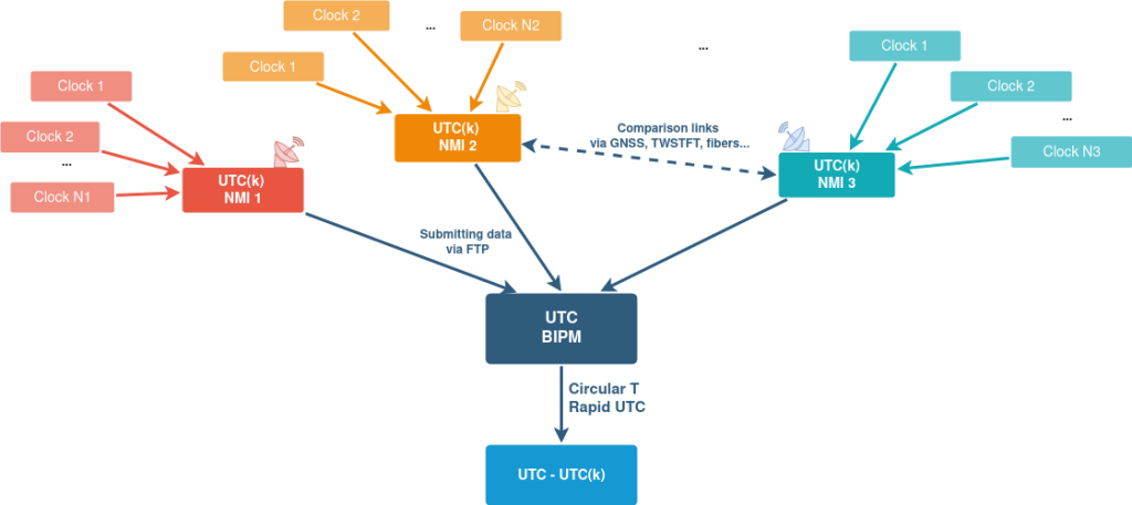
Figure 1: Creating UTC
However, TAI is a continuous atomic timescale, with no regard for the irregularities of Earth’s rotation. To maintain synchronisation with the natural day-night cycle, the International Earth Rotation Service (IERS) periodically introduces a leap second, aligning UTC to stay within 0.9 seconds of UT1, the astronomical time based on Earth’s actual rotation. At the moment of writing this entry, the total difference of TAI – UTC = 37 s. All leap seconds so far were positive, with the last one inserted on 31 December 2016. The potential application of a negative leap second in the future may be challenging, as it has never been applied so far.
As any leap second introduces a discontinuity in time, it can disrupt systems relying on continuous and monotonically increasing timestamps—a serious issue for Precision Time Protocol (PTP) implementations, where even sub-microsecond glitches can cause synchronisation errors or system instability. One example of how to test your NTP/PTP equipment by simulating a leap second can be found here.
While discussions of the future use of leap seconds continue, UTC remains the globally accepted compromise between the stable ticking of atomic clocks and the irregular, variable rotation of the Earth.
From Physics to Daily Life: Linking UTC to the Clock on Your Wall
The UTC timescale is defined as a “paper clock”—a mathematical result of clock comparison data analysis. True physical UTC realisation known as UTC(k) is generated by all k-participating NMIs, which tend to steer their timescales as close as possible to UTC. But how do you get it on your device?
This is where time dissemination comes in. There are several pathways. Some of them can establish direct connections to UTC(k) realisations, while most also involve service providers.
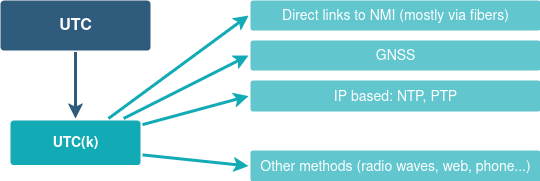
Figure 2: Dissemination methods
1. Direct Links to NMIs
Some institutions and industries (such as governmental and scientific facilities, telecom and power grid core networks, or finance) require the highest precision, reliability and traceability. They may establish direct timing links with NMIs, mostly using fibre-optic links, achieving synchronisation to within a few nanoseconds. These methods offer the best performance at higher costs.
2. Global Navigation Satellite Systems
Most modern time synchronisation relies on GNSS systems such as GPS, Galileo, BeiDou, or GLONASS. Each GNSS maintains and disseminates its own time scale, usually linked to UTC(k) or closely aligned with UTC. GNSS receivers use signals from satellites to derive accurate time, accessible globally and used for everything from banks and stock exchanges, data centres, to electric grid and transport operations. Often mistakenly confused with UTC, GNSS is the most frequently used, globally available and free time dissemination method, but GPS or GNSS generally is not a reference timescale. Also, all GNSS systems suffer from jamming and spoofing risks.
3. Network-Based Dissemination: NTP and PTP
For IP networks, Network Time Protocol (NTP) and Precision Time Protocol (PTP, IEEE 1588) are commonly used. NTP can synchronise computers and smartphones over the internet to within milliseconds, while PTP can achieve sub-microsecond-level precision over dedicated local networks. These protocols often rely on servers that are themselves synchronised via GNSS, atomic clocks or links to an NMI.
4. Other methods
There are also alternative options to access everyday information about the current “time of day”. One possibility is utilising long-wave radio signals to synchronise home “radio-controlled clocks” or even clocks in bigger organisations. An example of these systems is German DCF77, which covers most of Europe. Other options include access to “real-time” clocks via websites or phone services.
Bridging Science and Application
As the world becomes increasingly reliant on precise time—especially in sectors like 5G, finance, autonomous systems, and power grids—robust, secure, and accurate dissemination infrastructure is essential. From GNSS receivers and PTP Grandmaster clocks to high-stability NTP servers and modular time distribution systems, Meinberg provides the solutions that bring UTC from its source into your control room. Whether your need is millisecond accuracy for IT systems or nanosecond-level synchronisation for the highest-performance solutions or scientific research, Meinberg solutions offer the reliability and precision your applications demand.
Although there are many combinations of how to get accurate and traceable time to your application, one example is shown in Figure 3.
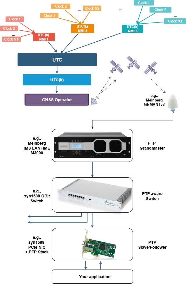
Figure 3: One example of getting time to your application
Please note that the GNSS system is here symbolically shown without going into details right away, this will be covered by another blog entry.
Disclaimer
We strive to ensure that all information published here is accurate and from verifiable sources. However, we cannot always guarantee that all details are up to date. Please, always double-check it when using it for further research.
If you enjoyed this post, or have any questions left, feel free to leave a comment or question below.